Quick Start

Here we present a step-by-step tutorial on the use of histolab to extract a tile dataset from example WSIs. The corresponding Jupyter Notebook is available at https://github.com/histolab/histolab-box: this repository contains a complete histolab environment that can be used through Docker on all platforms.

Thus, the user can decide either to use histolab through histolab-box or installing it in his/her python virtual environment (using conda, pipenv, pyenv, virtualenv, etc…). In the latter case, as the histolab package has been published on PyPI, it can be easily installed via the command:

pip install histolab

alternatively, it can be installed via conda:

conda install -c conda-forge histolab

TCGA data

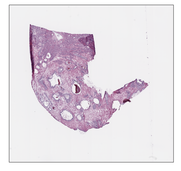
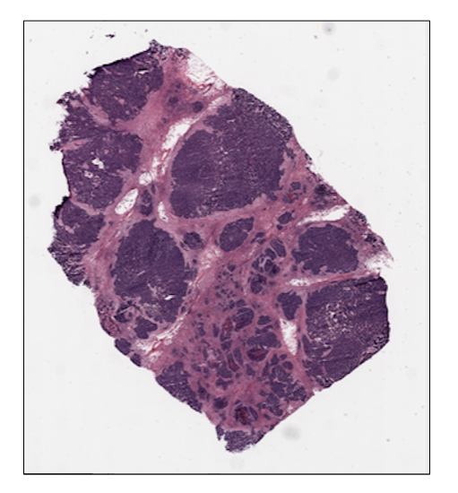
First things first, let’s import some data to work with, for example the prostate tissue slide and the ovarian tissue slide available in the data module:

from histolab.data import prostate_tissue, ovarian_tissue

Note: To use the data module, you need to install pooch, also available on PyPI (https://pypi.org/project/pooch/). This step is needless if we are using the Vagrant/Docker virtual environment.

The calling to a data function will automatically download the WSI from the corresponding repository and save the slide in a cached directory:

prostate_svs, prostate_path = prostate_tissue()
ovarian_svs, ovarian_path = ovarian_tissue()

Notice that each data function outputs the corresponding slide, as an OpenSlide object, and the path where the slide has been saved.

Slide initialization

histolab maps a WSI file into a Slide object. Each usage of a WSI requires a 1-o-1 association with a Slide object contained in the slide module:

from histolab.slide import Slide

To initialize a Slide it is necessary to specify the WSI path, and the processed_path where the tiles will be saved. In our example, we want the processed_path of each slide to be a subfolder of the current working directory:

import os

BASE_PATH = os.getcwd()

PROCESS_PATH_PROSTATE = os.path.join(BASE_PATH, 'prostate', 'processed')
PROCESS_PATH_OVARIAN = os.path.join(BASE_PATH, 'ovarian', 'processed')

prostate_slide = Slide(prostate_path, processed_path=PROCESS_PATH_PROSTATE)
ovarian_slide = Slide(ovarian_path, processed_path=PROCESS_PATH_OVARIAN)

Note: If the slides were stored in the same folder, this can be done directly on the whole dataset by using the SlideSet object of the slide module.

With a Slide object we can easily retrieve information about the slide, such as the slide name, the number of available levels, the dimensions at native magnification or at a specified level:

print(f"Slide name: {prostate_slide.name}")
print(f"Levels: {prostate_slide.levels}")
print(f"Dimensions at level 0: {prostate_slide.dimensions}")
print(f"Dimensions at level 1: {prostate_slide.level_dimensions(level=1)}")
print(f"Dimensions at level 2: {prostate_slide.level_dimensions(level=2)}")

Slide name: 6b725022-f1d5-4672-8c6c-de8140345210
Levels: [0, 1, 2]
Dimensions at level 0: (16000, 15316)
Dimensions at level 1: (4000, 3829)
Dimensions at level 2: (2000, 1914)

print(f"Slide name: {ovarian_slide.name}")
print(f"Levels: {ovarian_slide.levels}")
print(f"Dimensions at level 0: {ovarian_slide.dimensions}")
print(f"Dimensions at level 1: {ovarian_slide.level_dimensions(level=1)}")
print(f"Dimensions at level 2: {ovarian_slide.level_dimensions(level=2)}")

Slide name: b777ec99-2811-4aa4-9568-13f68e380c86
Levels: [0, 1, 2]
Dimensions at level 0: (30001, 33987)
Dimensions at level 1: (7500, 8496)
Dimensions at level 2: (1875, 2124)

Note

If the native magnification, i.e., the magnification factor used to scan the slide, is provided in the slide properties, it is also possible to convert the desired level to its corresponding magnification factor with the level_magnification_factor property.

print(
     "Native magnification factor:",
     prostate_slide.level_magnification_factor()
 )

 print(
     "Magnification factor corresponding to level 1:",
     prostate_slide.level_magnification_factor(level=1),
 )

Native magnification factor: 20X
Magnification factor corresponding to level 1: 5.0X

Moreover, we can retrieve or show the slide thumbnail in a separate window:

prostate_slide.thumbnail
prostate_slide.show()

ovarian_slide.thumbnail
ovarian_slide.show()

Tile extraction

Once that the Slide objects are defined, we can proceed to extract the tiles. To speed up the extraction process, histolab automatically detects the tissue region with the largest connected area and crops the tiles within this field. The tiler module implements different strategies for the tiles extraction and provides an intuitive interface to easily retrieve a tile dataset suitable for our task. In particular, each extraction method is customizable with several common parameters:

• tile_size: the tile size;

• level: the extraction level (from 0 to the number of available levels);

• check_tissue: if a minimum percentage of tissue is required to save the tiles;

• `` tissue_percent``: number between 0.0 and 100.0 representing the minimum required percentage of tissue over the total area of the image (default is 80.0)

• prefix: a prefix to be added at the beginning of the tiles’ filename (default is the empty string);

• suffix: a suffix to be added to the end of the tiles’ filename (default is .png).

Random Extraction

The simplest approach we may adopt is to randomly crop a fixed number of tiles from our slides; in this case, we need the RandomTiler extractor:

from histolab.tiler import RandomTiler

Let us suppose that we want to randomly extract 30 squared tiles at level 2 of size 128 from our prostate slide, and that we want to save them only if they have at least 80% of tissue inside. We then initialize our RandomTiler extractor as follows:

random_tiles_extractor = RandomTiler(
    tile_size=(128, 128),
    n_tiles=30,
    level=2,
    seed=42,
    check_tissue=True, # default
    tissue_percent=80.0, # default
    prefix="random/", # save tiles in the "random" subdirectory of slide's processed_path
    suffix=".png" # default
)

Notice that we also specify the random seed to ensure the reproducibility of the extraction process.

We may want to check which tiles have been selected by the tiler, before starting the extraction procedure and saving them; the locate_tiles method of RandomTiler returns a scaled version of the slide with the corresponding tiles outlined. It is also possible to specify the transparency of the background slide, and the color used for the border of the tiles:

random_tiles_extractor.locate_tiles(
    slide=prostate_slide,
    scale_factor=24,  # default
    alpha=128,  # default
    outline="red",  # default
)

Starting the extraction is then as simple as calling the extract method on the extractor, passing the slide as parameter:

random_tiles_extractor.extract(prostate_slide)

Random tiles extracted from the prostate slide at level 2.

Grid Extraction

Instead of picking tiles at random, we may want to retrieve all the tiles available. The Grid Tiler extractor crops the tiles following a grid structure on the largest tissue region detected in the WSI:

from histolab.tiler import GridTiler

In our example, we want to extract squared tiles at level 0 of size 512 from our ovarian slide, independently of the amount of tissue detected. By default, tiles will not overlap, namely the parameter defining the number of overlapping pixels between two adjacent tiles, pixel_overlap, is set to zero:

grid_tiles_extractor = GridTiler(
   tile_size=(512, 512),
   level=0,
   check_tissue=True, # default
   pixel_overlap=0, # default
   prefix="grid/", # save tiles in the "grid" subdirectory of slide's processed_path
   suffix=".png" # default
)

Again, we can exploit the locate_tiles method to visualize the selected tiles on a scaled version of the slide:

grid_tiles_extractor.locate_tiles(
    slide=ovarian_slide,
    scale_factor=64,
    alpha=64,
    outline="#046C4C",
)

and the extraction process starts when the extract method is called on our extractor:

grid_tiles_extractor.extract(ovarian_slide)

Examples of non-overlapping grid tiles extracted from the ovarian slide at level 0.

Score-based extraction

Depending on the task we will use our tile dataset for, the extracted tiles may not be equally informative. The ScoreTiler allows us to save only the “best” tiles, among all the ones extracted with a grid structure, based on a specific scoring function. For example, let us suppose that our goal is the detection of mitotic activity on our ovarian slide. In this case, tiles with a higher presence of nuclei are preferable over tiles with few or no nuclei. We can leverage the NucleiScorer function of the scorer module to order the extracted tiles based on the proportion of the tissue and of the hematoxylin staining. In particular, the score is computed as \(N_t\cdot\mathrm{tanh}(T_t)\), where \(N_t\) is the percentage of nuclei and \(T_t\) the percentage of tissue in the tile \(t\).

First, we need the extractor and the scorer:

from histolab.tiler import ScoreTiler
from histolab.scorer import NucleiScorer

As the ScoreTiler extends the GridTiler extractor, we also set the pixel_overlap as additional parameter. Moreover, we can specify the number of the top tiles we want to save with the n_tile parameter:

scored_tiles_extractor = ScoreTiler(
    scorer = NucleiScorer(),
    tile_size=(512, 512),
    n_tiles=100,
    level=0,
    check_tissue=True,
    tissue_percent=80.0,
    pixel_overlap=0, # default
    prefix="scored/", # save tiles in the "scored" subdirectory of slide's processed_path
    suffix=".png" # default
)

Notice that also the ScoreTiler implements the locate_tiles method, which visualizes (on a scaled version of the slide) the first n_tiles with the highest scores:

grid_tiles_extractor.locate_tiles(slide=ovarian_slide)

Finally, when we extract our cropped images, we can also write a report of the saved tiles and their scores in a CSV file:

summary_filename = "summary_ovarian_tiles.csv"
SUMMARY_PATH = os.path.join(ovarian_slide.processed_path, summary_filename)

scored_tiles_extractor.extract(ovarian_slide, report_path=SUMMARY_PATH)

Representation of the score assigned to each extracted tile by the NucleiScorer, based on the amount of nuclei detected.